1 An overview of machine learning and deep learning
This chapter covers
- A first look at machine learning and deep learning
- A simple machine learning model: The cat brain
- Understanding deep neural networks
Deep learning has transformed computer vision, natural language and speech processing in particular, and artificial intelligence in general. From a bag of semi-discordant tricks, none of which worked satisfactorily on real-life problems, artificial intelligence has become a formidable tool to solve real problems faced by industry, at scale. This is nothing short of a revolution going on under our very noses. To lead the curve of this revolution, it is imperative to understand the underlying principles and abstractions rather than simply memorizing the “how-to” steps of some hands-on guide. This is where mathematics comes in.
In this first chapter, we present an overview of deep learning. This will require us to use some concepts explained in subsequent chapters. Don’t worry if there are some open questions at the end of this chapter: it is aimed at orienting your mind toward this difficult subject. As individual concepts become clearer in subsequent chapters, you should consider coming back and re-reading this chapter.
1.1 A first look at machine/deep learning: A paradigm shift in computation
Making decisions and/or predictions is a central requirement of life. Doing so essentially involves taking in a set of sensory or knowledge inputs and processing them to generate decisions or estimates.
For instance, a cat’s brain is often trying to choose between the following options:
-
run away from the object in front of it
-
ignore the object in front of it
-
approach the object in front of it and purr.
The cat’s brain makes that decision by processing sensory inputs like the perceived hardness of the object in front of it, the perceived sharpness of the object in front of it, and so on. This is an instance of a classification problem, where the output is one of a set of possible classes.
Some other examples of classification problems in life are as follows:
-
Buy vs. hold vs. sell a certain stock, from inputs like the price history of this stock and the change in price of the stock in recent times
-
Object recognition (from an image):
-
Is this a car or a giraffe?
-
Is this a human or a non-human?
-
Is this an inanimate object or a living object?
-
Face recognition—is this Tom or Dick or Mary or Einstein or Messi?
-
-
Action recognition from a video:
-
Is this person running or not running?
-
Is this person picking something up or not?
-
Is this person doing something violent or not?
-
-
Natural language processing (NLP) from digital documents:
-
Does this news article belong to the realm of politics or sports?
-
Does this query phrase match a particular article in the archive?
-
Sometimes life requires a quantitative estimation instead of a classification. A lion’s brain needs to estimate how far to jump so as to land on top of its prey, by processing inputs like
Another instance of quantitative estimation is estimating a house’s price based on inputs like current income of the house’s owner, crime statistics for the neighborhood, and so on. Machines that make such quantitative estimators are called regressors.
Here are some other examples of quantitative estimations required in daily life:
-
Object localization from an image: identifying the rectangle bounding the location of an object
-
Stock price prediction from historical stock prices and other world events
-
Similarity score between a pair of documents
Sometimes a classification output can be generated from a quantitative estimate. For instance, the cat brain described earlier can combine the inputs (hardness, sharpness, and so on) to generate a quantitative threat score. If that threat score is high, the cat runs away. If the threat score is near zero, the cat ignores the object in front of it. If the threat score is negative, the cat approaches the object and purrs.
Many of these examples are shown in figure 1.1. In each instance, a machine—that is, a brain—transforms sensory or knowledge inputs into decisions or quantitative estimates. The goal of machine learning is to emulate that machine.
Note that machine learning has a long way to go before it can catch up with the human brain. The human brain can single-handedly deal with thousands, if not millions, of such problems. On the other hand, at its present state of development, machine learning can hardly create a single general-purpose machine that makes a wide variety of decisions and estimates. We are mostly trying to make separate machines to solve individual tasks (such as a stock picker or a car recognizer).
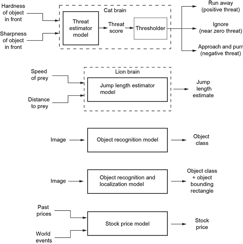
Figure 1.1 Examples of decision making and quantitative estimations in life
At this point, you may ask, “Wait: converting inputs to outputs—isn’t that exactly what computers have been doing for the last 30 or more ears? What is this paradigm shift I am hearing about?” The answer is that it is a paradigm shift because we do not provide a step-by-step instruction set—that is, a program—to the machine to convert the input to output. Instead, we develop a mathematical model for the problem.
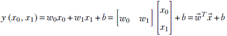
Let’s illustrate the idea with an example. For the sake of simplicity and concreteness, we will consider a hypothetical cat brain that needs to make only one decision in life: whether to run away from the object in front of it or ignore the object or approach and purr. This decision, then, is the output of the model we will discuss. And in this toy example, the decision is made based on only two quantitative inputs (aka features): the perceived hardness and sharpness of the object (as depicted in figure 1.1). We do not provide any step-by-step instructions such as “if sharpness greater than some threshold, then run away.” Instead, we try to identify a parameterized function that takes the input and converts it to the desired decision or estimate. The simplest such function is a weighted sum of inputs:
y(hardness, sharpness) = w0 × hardness + w1 × sharpness + b
The weights w0, w1 and the bias b are the parameters of the function. The output y can be interpreted as a threat score. If the threat score exceeds a threshold, the cat runs away. If it is close to 0, the cat ignores the object. If the threat score is negative, the cat approaches and purrs. For more complex tasks, we will use more sophisticated functions.
Note that the weights are not known at first; we need to estimate them. This is done through a process called model training.
Overall, solving a problem via machine learning has the following stages:
-
We design a parameterized model function (e.g., weighted sum) with unknown parameters (weights). This constitutes the model architecture. Choosing the right model architecture is where the expertise of the machine learning engineer comes into play.
-
Then we estimate the weights via model training.
-
Once the weights are estimated, we have a complete model. This model can take arbitrary inputs not necessarily seen before and generate outputs. The process in which a trained model processes an arbitrary real-life input and emits an output is called inferencing.
In the most popular variety of machine learning, called supervised learning, we prepare the training data before we commence training. Training data comprises example input items, each with its corresponding desired output. 1 Training data is often created manually: a human goes over every single input item and produces the desired output (aka target output). This is usually the most arduous part of doing machine learning.
For instance, in our hypothetical cat brain example, some possible training data items are as follows
input: hardness = 0.01, sharpness = 0.02 → threat = —0.90 → decision: “approach and purr”
input: hardness = 0.50, sharpness = 0.60 → threat = 0.01 → decision: “ignore”
input: hardness = 0.99, sharpness = 0.97 → threat = 0.90 → decision: “run away”
where the input values of hardness and sharpness are assumed to lie between 0 and 1.
What exactly happens during training? Answer: we iteratively process the input training data items. For each input item, we know the desired aka target) output. On each iteration, we adjust the model weight values in a way that the output of the model function on that specific input item gets at least a little closer to the corresponding target output. For instance, suppose at a given iteration, the weight values are w0 = 20 and w1 = 10, and b = 50. On the input (hardness = 0.01, sharpness = 0.02), we get an output threat score y = 50.3, which is quite different from the desired y = −0.9. We will adjust the weights: for instance, reducing the bias so w0 = 20, w1 = 10, and b = 40. The corresponding threat score y = 40.3 is still nowhere near the desired value, but it has moved closer. After we do this on many training data items, the weights will start approaching their ideal values. Note that how to identify the adjustments to the weight values is not discussed here; it requires somewhat deeper math and will be discussed later.
As stated earlier, this process of iteratively tuning weights is called training or learning. At the beginning of learning, the weights have random values, so the machine outputs often do not match desired outputs. But with time, more training iterations happen, and the machine “learns” to generate the correct output. That is when the model is ready for deployment in the real world. Given arbitrary input, the model will (hopefully) emit something close to the desired output during inferencing.
Come to think of it, that is probably how living brains work. They contain equivalents of mathematical models for various tasks. Here, the weights are the strengths of the connections (aka synapses) between the different neurons in the brain. In the beginning, the parameters are untuned; the brain repeatedly makes mistakes. For example, a baby’s brain often makes mistakes in identifying edible objects—anybody who has had a child will know what we are talking about. But each example tunes the parameters (eating green and white rectangular things with a $ sign on them invites much scolding—should not eat them in the future, etc.). Eventually, this machine tunes its parameters to yield better results.
One subtle point should be noted here. During training, the machine is tuning its parameters so that it produces the desired outcome—on the training data input only. Of course, it sees only a small fraction of all possible inputs during training—we are not building a lookup table from known inputs to known outputs. Hence, when this machine is released in the world, it mostly runs on input data it has never seen before. What guarantee do we have that it will generate the right outcome on never-before-seen data? Frankly, there is no guarantee. Only, in most real-life problems, the inputs are not really random. They have a pattern. Hopefully, the machine will see enough during training to capture that pattern. Then its output on unseen input will be close to the desired value. The closer the distribution of the training data is to real life, the more likely that becomes.
1.2 A function approximation view of machine learning:Models and their training
As stated in section 1.1, to create a brain-like machine that makes classifications or estimations, we have to find a mathematical function (model) that transforms inputs into corresponding desired outputs. Sadly, however, in typical real-life situations, we do not know that transformation function. For instance, we do not know the function that takes in past prices, world events, and so on and estimates the future price of a stock—something that stops us from building a stock price estimator and getting rich. All we have is the training data—a set of inputs on which the output is known. How do we proceed, then? Answer: we will try to model the unknown function. This means we will create a function that will be a proxy or surrogate to the unknown function. Viewed this way, machine learning is nothing but function approximation—we are simply trying to approximate the unknown classification or estimation function.
Let’s briefly recap the main ideas from the previous section. In machine learning, we try to solve problems that can be abstractly viewed as transforming a set of inputs to an output. The output is either a class or an estimated value. Since we do not know the true transformation function, we try to come up with a model function. We start by designing—using our physical understanding of the problem—a model function with tunable parameter values that can serve as a proxy for the true function. This is the model architecture, and the tunable parameters are also known as weights. The simplest model architecture is one where the output is a weighted sum of the input values. Determining the model architecture does not fully determine the model—we still need to determine the actual parameter values (weights). That is where training comes in. During training, we find an optimal set of weights that transform the training inputs to outputs that match the corresponding training outputs as closely as possible. Then we deploy this machine in the world: its weights are estimated and the function is fully determined, so on any input, it simply applies the function and generates an output. This is called inferencing. Of course, training inputs are only a fraction of all possible inputs, so there is no guarantee that inferencing will yield a desired result on all real inputs. The success of the model depends on the appropriateness of the chosen model architecture and the quality and quantity of training data.
Now, let’s study the process of model building with a concrete example: the cat brain machine shown in figure 1.1.
1.3 A simple machine learning model: The cat brain
For the sake of simplicity and concreteness, we will deal with a hypothetical cat that needs to make only one decision in life: whether to run away from the object in front of it, ignore it, or approach and purr. And it makes this decision based on only two quantitative inputs pertaining to the object in front of it (shown in figure 1.1).
NOTE This chapter is a lightweight overview of machine/deep learning. As such, it relies some on mathematical concepts that we will introduce later. You are encouraged to read this chapter now, nonetheless, and perhaps re-read it after digesting the chapters on vectors and matrices.
1.3.1 Input features
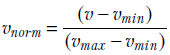
The input features are x0, signifying hardness, and x1, signifying sharpness. Without loss of generality, we can normalize the inputs. This is a pretty popular trick whereby the input values ranging between a minimum possible value vmin and a maximum possible value vmax are transformed to values between 0 and 1. To transform an arbitrary input value v to a normalized value vnorm, we use the formula
Equation 1.1
In mathematical parlance, transformation via equation 1.1, v ∈ [vmin, vmax] → vnorm ∈ [0,1] maps the values v from the input domain [vmin, vmax] to the output values vnorm in the range [0,1].
A two-element vector  represents a single input instance succinctly.
1.3.2 Output decisions
The final output is multiclass and can take one of three possible values: 0, implying running away from the object in front of the cat; 1, implying ignoring the object; and 2, implying approaching the object and purring. It is possible in machine learning to compute the class directly. However, in this example, we will have our model estimate a threat score. It is interpreted as follows: threat high positive = run away, threat near zero = ignore, and threat high negative = approach and purr (negative threat is attractive).
We can make a final multiclass run/ignore/approach decision based on threat score by comparing the threat score y against a threshold δ, as follows:
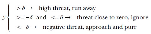
Equation 1.2
1.3.3 Model estimation
Now for the all-important step: we need to estimate the function that transforms the input vector to the output. With slight abuse of terms, we will denote this function as well as the output by y. In mathematical notation, we want to estimate y(![]() ).
).
Of course, we do not know the ideal function. We will try to estimate this unknown function from the training data. This is accomplished in two steps:
-
Model architecture selection—Designing a parameterized function that we expect is a good proxy or surrogate for the unknown ideal function
-
Training—Estimating the parameters of that chosen function such that the outputs on training inputs match corresponding outputs as closely as possible
1.3.4 Model architecture selection
This is the step where various machine learning approaches differ from one another. In this toy cat brain example, we will use the simplest possible model. Our model has three parameters, w0, w1, b. They can be represented compactly with a single two-element vector  and a constant bias b ∈ ℝ (here, ℝ denotes the set of all real numbers, ℝ2 denotes the set of 2D vectors with both elements real, and so on). It emits the threat score, y, which is computed as
Equation 1.3
Note that b is a slightly special parameter. It is a constant that does not get multiplied by any of the inputs. It is common practice in machine learning to refer to it as bias; the other parameters are multiplied by inputs as weights.
1.3.5 Model training
Once the model architecture is chosen, we know the exact parametric function we are going to use to model the unknown function y(![]() ) that transforms inputs to outputs. We still need to estimate the function’s parameters. Thus, we have a function with unknown parameters, and the parameters are to be estimated from a set of inputs with known outputs (training data). We will choose the parameters so that the outputs on the training data inputs match the corresponding outputs as closely as possible.
) that transforms inputs to outputs. We still need to estimate the function’s parameters. Thus, we have a function with unknown parameters, and the parameters are to be estimated from a set of inputs with known outputs (training data). We will choose the parameters so that the outputs on the training data inputs match the corresponding outputs as closely as possible.
Concretely, the goal of the training process is to estimate the parameters w0, w1, b or, equivalently, the vector ![]() along with constant b from equation 1.3 in such a way that the output y(x0, x1) on the training data input (x0, x1) matches the corresponding known training data outputs (aka ground truth [GT]) as much as possible.
along with constant b from equation 1.3 in such a way that the output y(x0, x1) on the training data input (x0, x1) matches the corresponding known training data outputs (aka ground truth [GT]) as much as possible.
Let the training data consist of N + 1 inputs ![]() (0),
(0), ![]() (1), ⋯
(1), ⋯ ![]() (N). Here, each
(N). Here, each ![]() (i) is a 2 × 1 vector denoting a single training data input instance. The corresponding desired threat values (outputs) are ygt(0), ygt(1), ⋯ ygt(N), say (here, the subscript gt denotes ground truth). Equivalently, we can say that the training data consists of N + 1 (input, output) pairs:
(i) is a 2 × 1 vector denoting a single training data input instance. The corresponding desired threat values (outputs) are ygt(0), ygt(1), ⋯ ygt(N), say (here, the subscript gt denotes ground truth). Equivalently, we can say that the training data consists of N + 1 (input, output) pairs:
(![]() (0), ygt(0)), (
(0), ygt(0)), (![]() (1), ygt(1))⋯(
(1), ygt(1))⋯(![]() (N), ygt(N))
(N), ygt(N))
Suppose ![]() denotes the (as-yet-unknown) optimal parameters for the model. Then, given an arbitrary input
denotes the (as-yet-unknown) optimal parameters for the model. Then, given an arbitrary input ![]() , the machine will estimate a threat value of ypredicted =
, the machine will estimate a threat value of ypredicted = ![]() T
T![]() + b. On the ith training data pair, (
+ b. On the ith training data pair, (![]() (i), ygt(i)) the machine will estimate
(i), ygt(i)) the machine will estimate
ypredicted(i) = ![]() T
T![]() (i) + b
(i) + b
while the desired output is ygt(i). Thus the squared error (aka loss) made by the machine on the ith training data instance is 2
ei2 = (ypredicted(i)−ygt(i))2
The overall loss on the entire training data set is obtained by adding the loss from each individual training data instance:
The goal of training is to find the set of model parameters (aka weights), ![]() , that minimizes the total error E. Exactly how we do this will be described later.
, that minimizes the total error E. Exactly how we do this will be described later.
In most cases, it is not possible to come up with a closed-form solution for the optimal ![]() , b. Instead, we take an iterative approach depicted in algorithm 1.1.
, b. Instead, we take an iterative approach depicted in algorithm 1.1.
Algorithm 1.1 Training a supervised model
Initialize parameters ![]() , b with random values
, b with random values
⊳ iterate while error not small enough
while (E2 = Σi = 0i=N (![]() T
T![]() i ¸ b — ygt(i))2 > threshold) do
i ¸ b — ygt(i))2 > threshold) do
⊳ iterate over all training data instances
for ∀i ∈ 2 [0, N] do
⊳ details provided in section 3.3 after gradients are introduced
Adjust ![]() , b so that E2 is reduced
, b so that E2 is reduced
end for
end while
⊳ remember the final parameter values as optimal
![]() *←
*← ![]() , b*← b
, b*← b
In this algorithm, we start with random parameter values and keep tuning the parameters so the total error goes down at least a little. We keep doing this until the error becomes sufficiently small.
In a purely mathematical sense, we continue the iterations until the error is minimal. But in practice, we often stop when the results are accurate enough for the problem being solved. It is worth re-emphasizing that error here refers only to error on training data.
1.3.6 Inferencing
Finally, a trained machine (with optimal parameters ![]() *, b* is deployed in the world. It will receive new inputs
*, b* is deployed in the world. It will receive new inputs ![]() and will infer ypredicted(
and will infer ypredicted(![]() ) =
) = ![]() *T
*T![]() + b*. Classification will happen by thresholding ypredicted, as shown in equation 1.2.
+ b*. Classification will happen by thresholding ypredicted, as shown in equation 1.2.
1.4 Geometrical view of machine learning
Each input to the cat brain model is an array of two numbers: x0 (signifying hardness of the object), x1 signifying sharpness of the object) or, equivalently, a 2 × 1 vector ![]() . A good mental picture is to think of the input as a point in a high-dimensional space. The input space is often called the feature space—a space where all the characteristic features to be examined by the model are represented. The feature space dimension is two in this case, but in real-life problems it will be in the hundreds or thousands or more. The exact dimensionality of the input changes from problem to problem, but the intuition that it is a point remains.
. A good mental picture is to think of the input as a point in a high-dimensional space. The input space is often called the feature space—a space where all the characteristic features to be examined by the model are represented. The feature space dimension is two in this case, but in real-life problems it will be in the hundreds or thousands or more. The exact dimensionality of the input changes from problem to problem, but the intuition that it is a point remains.
The output y should also be viewed as a point in another high-dimensional space. In this toy problem, the dimensionality of the output space is one, but in real problems, it will be higher. Typically, however, the number of output dimensions is much smaller than the number of input dimensions.
Geometrically speaking, a machine learning model essentially maps a point in the feature space to a point in the output space. It is expected that the classification or estimation job to be performed by the model is easier in the output space than in the feature space. In particular, for a classification job, input points belonging to separate classes are expected to map to separate clusters in output space.
Let’s continue with our example cat brain model to illustrate the idea. As stated earlier, our feature space is 2D, with two coordinate axes X0 signifying hardness and X1 signifying sharpness.3 Individual points in this 2D space are denoted by coordinate values (x0, x1) in lowercase (see figure 1.2). As shown in the diagram, a good way to model the threat score is to measure the distance from line x0 + x1 = 1.
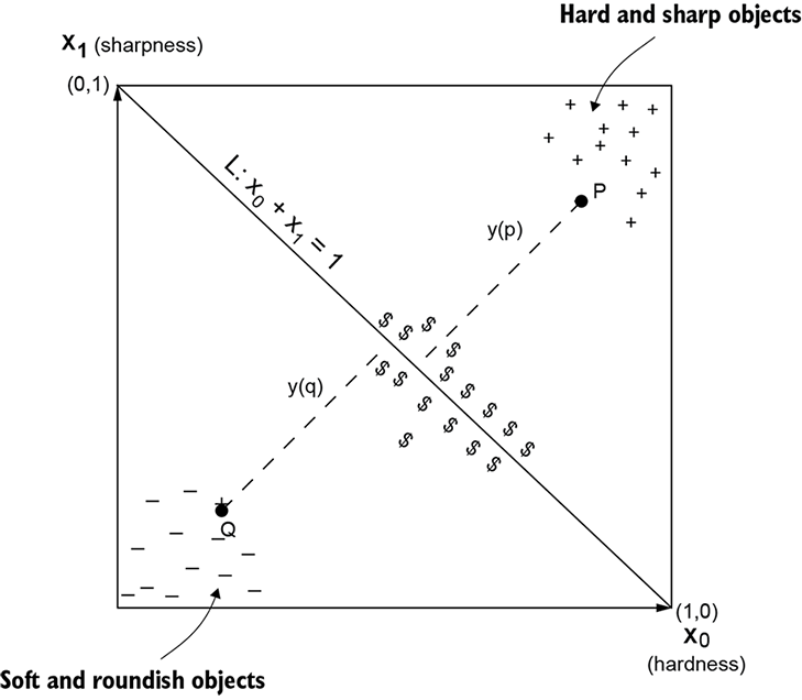
Figure 1.2 2D input point space for the cat brain model. The bottom-left corner shows objects with low hardness and low sharpness objects (–), while the top-right corner shows objects with high hardness and high sharpness (+). Intermediate values are near the diagonal ($).
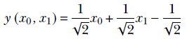
From coordinate geometry, in a 2D space with coordinate axes X0 and X1, the signed distance of a point (a, b) from the line x0 + x1 = 1 is y = (a+b–1)/√2. Examining the sign of y, we can determine which side of the separator line the input point belongs to. In the simple situation depicted in figure 1.2, observation tells us that the threat score can be proxied by the signed distance, y, from the diagonal line x0 + x1 – 1 = 0. We can make the run/ignore/approach decision by thresholding y. Values close to zero imply ignore, positive values imply run away, and negative values imply approach and purr. From high school geometry, the distance of an arbitrary input point (x0=a, x1=b) from line x0 + x1 – 1 = 0 is (a+b–1)/√2. Thus, the function y(x0, x1) = (x0 + x1–1)/√2 is a possible model for the cat brain threat estimator function. Training should converge to w0 = 1/√2, w1 = 1/√2 and b = –1/√2.
Thus, our simplified cat brain threat score model is
Equation 1.4
It maps the 2D input points, signifying the hardness and sharpness of the object in front of the cat, to a 1D value corresponding to the signed distance from a separator line. This distance, physically interpretable as a threat score, makes it possible to separate the classes (negative threat, neutral, positive threat) via thresholding, as shown in equation 1.2. The separate classes form distinct clusters in the output space, depicted by +, –, and $ signs in the output space. Low values of inputs produce negative threats (the cat will approach and purr): for example, y(0, 0) = –1/√2. High values of inputs produce high threats (the cat will run away): for example, y(1, 1) = 1/√2. Medium values of inputs produce near-zero threats (the cat will ignore the object): for example, y(0.5, 0.5) = 0. Of course, because the problem is so simple, we could come up with the model parameters via simple observation. In real-life situations, this will need training.
The geometric view holds in higher dimensions, too. In general, an n-dimensional input vector ![]() is mapped to an m-dimensional output vector (usually m < n) in such a way that the problem becomes much simpler in the output space. An example with 3D feature space is shown in figure 1.3.
is mapped to an m-dimensional output vector (usually m < n) in such a way that the problem becomes much simpler in the output space. An example with 3D feature space is shown in figure 1.3.
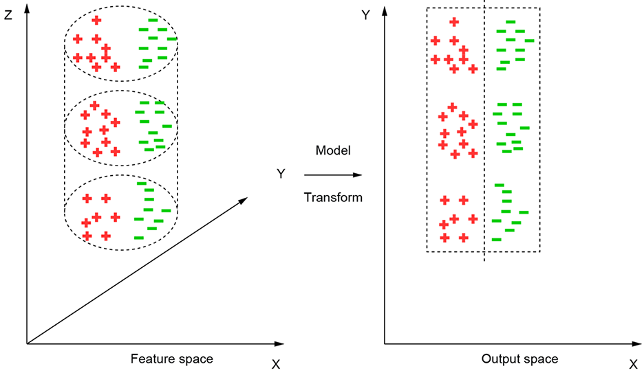
Figure 1.3 A model maps the points from input (feature) space to an output space where it is easier to separate the classes. For instance, in this figure, input feature points belonging to two classes, red (+) and green (–) are distributed over the volume of a cylinder in a 3D feature space. The model unfurls the cylinder into a rectangle. The feature points are mapped onto a 2D planar output space where the two classes can be discriminated with a simple linear separator.
Figure 1.4 The two classes (indicated by light and dark shades) cannot be separated by a line. A curved separator is needed. In 3D, this is equivalent to saying that no plane can separate the surfaces; a curved surface is necessary. In still higher-dimensional spaces, this is equivalent to saying that no hyperplane can separate the classes; a curved is needed.
1.5 Regression vs. classification in machine learning
As briefly outlined in section 1.1, there are two types of machine learning models: regressors and classifiers.
In a regressor, the model tries to emit a desired value given a specific input. For instance, the first stage (threat-score estimator) of the cat brain model in section 1.3 is a regressor model.
Classifiers, on the other hand, have a set of prespecified classes. Given a specific input, they try to emit the class to which the input belongs. For instance, the full cat brain model has three classes: 1) run away, (2) ignore, and (3) approach and purr. Thus, it takes an input (hardness and sharpness values) and emits an output decision (aka class).
In this example, we convert a regressor into a classifier by thresholding the output of the regressor (see equation 1.2). It is also possible to create models that directly output the class without having an intervening regressor.
1.6 Linear vs. nonlinear models
In figure 1.2 we faced a rather simple situation where the classes could be separated by a line (a hyperplane in higher-dimensional surfaces). This does not happen often in real life. What if the points belonging to different classes are as shown in figure 1.4? In such cases, our model architecture should no longer be a simple weighted combination. It is a nonlinear function. For instance, check the curved separator in figure 1.4. Nonlinear models make sense from the function approximation point of view as well. Ultimately, our goal is to approximate very complex and highly nonlinear functions that model the classification or estimation processes demanded by life. Intuitively, it seems better to use nonlinear functions to model them.
A very popular nonlinear function in machine learning is the sigmoid function, so named because it looks like the letter S. The sigmoid function is typically symbolized by the Greek letter σ. It is defined as
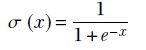
Equation 1.5
The graph of the sigmoid function is shown in figure 1.5. Thus we can use the following popular model architecture (still kind of simple) that takes the sigmoid without parameters) of the weighted sum of the inputs:
![]()
Equation 1.6
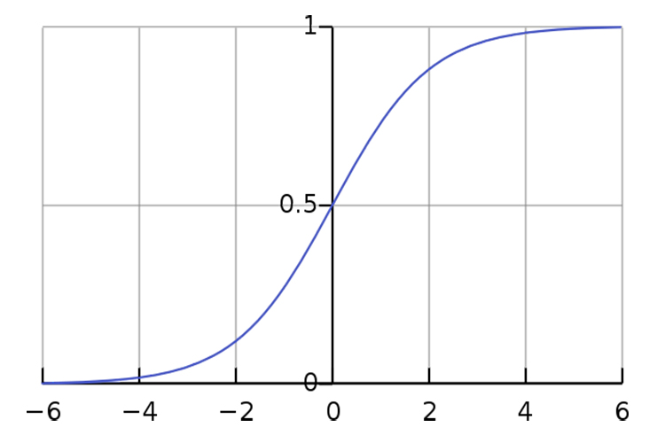
Figure 1.5 The sigmoid graph
The sigmoid imparts the nonlinearity. This architecture can handle relatively more complex classification tasks than the weighted sum alone. In fact, equation 1.6 depicts the basic building block of a neural network.
1.7 Higher expressive power through multiple nonlinear layers: Deep neural networks
In section 1.6 we stated that adding nonlinearity to the basic weighted sum yielded a model architecture that is able to handle more complex tasks. In machine learning parlance, the nonlinear model has more expressive power.
Now consider a real-life problem: say, building a dog recognizer. The input space comprises pixel locations and pixel colors (x, y, r, g, b, where r, g, b denote the red, green, and blue components of a pixel color). The input dimensionality is large (proportional to the number of pixels in the image). Figure 1.6 gives a small glimpse of the possible variations in background and foreground that a typical deep learning system (such as a dog image recognizer) has to deal with.
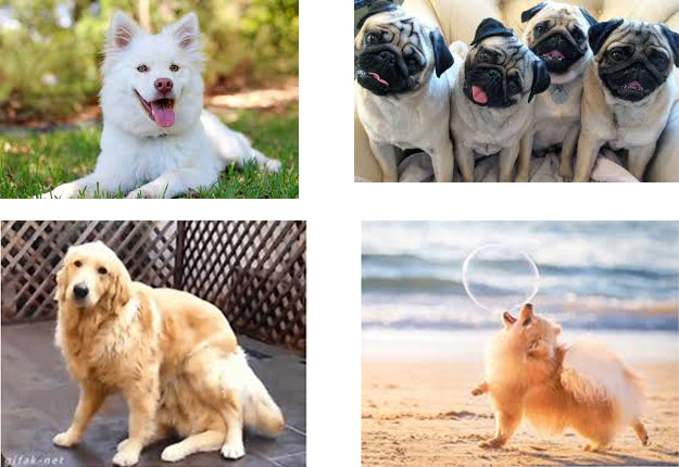
Figure 1.6 A glimpse into background and foreground variations that a typical deep learning system (here, a dog image recognizer) has to deal with
We need a machine with really high expressive power here. How do we create such a machine in a principled way?
Instead of generating the output from input in a single step, how about taking a cascaded approach? We will generate a set of intermediate or hidden outputs from the inputs, where each hidden output is essentially a single logistic regression unit. Then we add another layer that takes the output of the previous layer as input, and so on. Finally, we combine the outermost hidden layer outputs into the grand output.
We describe the system in the following equations. Note that we have added a superscript to the weights to identify the layer (layer 0 is closest to the input; layer L is the last layer, furthest from the input). We have also made the subscripts twodimensional (so the weights for a given layer become a matrix). The first subscript identifies the destination node, and the second subscript identifies the source node (see figure 1.7).
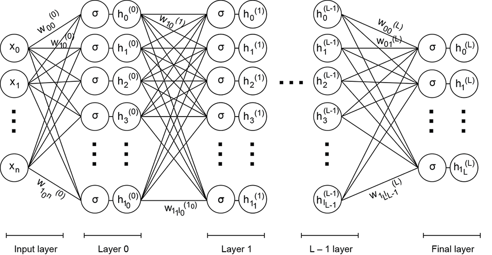
Figure 1.7 Multilayered neural network
The astute reader may notice that the following equations do not have an explicit bias term. That is because, for simplicity of notation, we have rolled it into the set of weights and assumed that one of the inputs (say, x0 = 1) and the corresponding weight (such as w0) is the bias.
Layer 0: generates n0 hidden outputs from n + 1 inputs
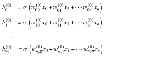
Equation 1.7
Layer 1: generates n1 hidden outputs from n0 hidden outputs from layer
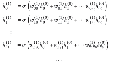
Equation 1.8
Final layer (L): generates m + 1 visible outputs from nL − 1 previous layer hidden outputs
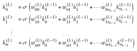
Equation 1.9
These equations are shown in figure 1.7. The machine depicted in figure 1.7 can be incredibly powerful, with huge expressive power. We can adjust its expressive power systematically to fit the problem at hand. It then is a neural network. We will devote the rest of the book to studying this.
Summary
In this chapter, we gave an overview of machine learning, leading all the way up to deep learning. The ideas were illustrated with a toy cat brain example. Some mathematical notions (e.g., vectors) were used in this chapter without proper introduction, and you are encouraged to revisit this chapter after vectors and matrices have been introduced.
We would like to leave you with the following mental pictures from this chapter:
-
Machine learning is a fundamentally different paradigm of computing. In traditional computing, we provide a step-by-step instruction sequence to the computer, telling it what to do. In machine learning, we build a mathematical model that tries to approximate the unknown function that generates a classification or estimation from inputs.
-
The mathematical nature of the model function is stipulated from the physical nature and complexity of the classification or estimation task. Models have parameters. Parameter values are estimated from training data—inputs with known outputs. The parameter values are optimized so that the model output is as close as possible to training outputs on training inputs.
-
An alternative geometric view of a machine is a transformation that maps points in the multidimensional input space to a point in the output space.
-
The more complex the classification/estimation task, the more complex the approximating function. In machine learning parlance, complex tasks need machines with greater expressive power. Higher expressive power comes from nonlinearity (e.g., the sigmoid function; see equation 1.5) and a layered combination of simpler machines. This takes us to deep learning, which is nothing but a multilayered nonlinear machine.
-
Complex model functions are often built by combining simpler basis functions.
Tighten your seat belts: the fun is about to get more intense.
1 If you have some experience with machine learning, you will realize that we are talking about “supervised” learning here. There are also machines that do not need known outputs to learn—so-called “unsupervised” machines—and we will talk about them later. ↩
2 In this context, note that it is a common practice to square the error/loss to make it sign independent. If we desire an output of, say, 10, we are equally happy/unhappy if the output is 9.5 or 10.5. Thus, an error of + 5 or −5 is effectively the same; hence we make the error sign independent. ↩
3 We use X0, X1 as coordinate symbols instead of the more familiar X, Y so as not to run out of symbols when going to higher-dimensional spaces. ↩
4 In mathematics, vectors can have an infinite number of elements. Such vectors cannot be expressed as arrays—but we will mostly ignore them in this book. ↩